Backgammon
Below are some notes on training a backgammon agent with TD learning.
Backgammon agents have been strong for a long time, and remarkably you only need a small model! TD-Gammon [3], old work from the 1990s, is decent using just a tiny 3-layer neural network.
Setup
For simplicity, we consider modelling only single cubeless games rather than multi-game matches.
We are interested in 'equity'. Equity is the expected number of points a player will get from the current position. In backgammon, there are two players, and the winning player will get either win 1, 2, or 3 points. We model these 6 outcomes as 6 probabilities from each input state $s$, $$ p_\theta(s) = [p_{0,1},\,p_{0,2},\,p_{0,3},\,p_{1,1},\,p_{1,2},\,p_{1,3}]^\top, $$ where $p_{i,j}$ is the probability that player $i$ wins $j$ points. Here $\theta$ represents the parameters, and we drop the $\theta$ subscript from $p_{i,j}$ for notational convenience. Player 0's equity is, $$ \begin{aligned} V_\theta(s) &= c^\top p_\theta(s)\\ \text{where}\quad c&=[1,2,3,-1,-2,-3]^\top \end{aligned} $$ We also refer to $V_\theta(\cdot)$ as the value function. Since backgammon is zero-sum, player 1's equity is simply $-V_\theta(s)$. Player 0 ideally tries to make moves that give the best equity, i.e.the game enters a state $s$ with high $V_\theta(s)$.
Note: maximizing $V_\theta$ might be undesirable vs. maximizing $p_{0,1}$ in specific circumstances. For example, in a match with 1 point to win going for a gammon or backgammon is riskier. But we ignore this subtlety for now.
TD learning
We give an overview of TD($\lambda$) in the context of backgammon below.
Bellman
Let $t$ index the different board states through time (i.e. $t$ indexes turns), and let $R_{t}$ be the reward received when entering $s_t$. In backgammon, $R_t = 0$ except at the very end of the game, call it time $T$, where we have $R_T = \pm 1/2/3$. We consider the value of the terminal state to be zero, i.e. $V(s_T) = 0$, with all the reward coming from $R_T$.
The Bellman equation says that the value of the current state is the immediate reward, in addition to the discounted value of the future state, $$ V(s_t) = \mathbb{E}[R_{t+1} + \gamma V(s_{t+1})]. $$ By $V$ we mean the 'true' value function, whereas by $V_\theta$ we mean our model. The scalar $\gamma \leq 1$ is the discount. The expectation is over both the action and environment, so more accurately, $$ V(s_t) =\mathbb{E}_{a\sim \pi(a\mid s_t)}\bigg[\mathbb{E}_{s_{t+1}\sim p_e(s_{t+1}\mid s_t,\,a)}[R_{t+1}(s_t,\,a,\,s_{t+1}) + \gamma V(s_{t+1})]\bigg]. $$ Here, the action $a$ is selected using the optimal policy $\pi$, and then the environment gives us a new state $s_{t+1}$ conditional on the action $a$ and the previous state $s_t$. In backgammon, the stochasticity of the environment (denoted by the distribution $p_e$) comes entirely from the dice.
In practice the Bellman equation will not be true for our model $V_\theta$, but it will become our train target! Given a rollout $s_1,\,\ldots,\,s_T$, we aim to minimize the following difference,
$$ \mathbb{E}_{a\sim \pi_\theta(a\mid s_t) ,\,s_{t+1}\sim p_e(s_{t+1}\mid a,\,s_t)}[R_{t+1} + \gamma V_\theta(s_{t+1})] - V_{\theta}(s_{t}). $$ where in lieu of the optimal policy $\pi$, we use a model $\pi_\theta$. For backgammon, we can cheaply compute $\pi_\theta$ by iterating over all possible moves $a$, and selecting the one which maximizes $V_\theta(s_{t+1})$.
The exact expectation (one-step) is actually feasible in backgammon but here we approximate it with the sample we have available. This gives the TD (temporal difference) error,
$$
\delta_t = R_{t+1} + \gamma V_\theta(s_{t+1}) - V_{\theta}(s_{t}).
$$
We treat $y =R_{t+1} + \gamma V_\theta(s_{t+1})$ as the target, and try to optimize $V_\theta(s_t)$ toward $y$. One gotcha is that the target also depends on the parameters, so we apply stopgrad to $y$.
TD vs. TD($\lambda$) vs. full Monte Carlo rollout
Above we said we can try to minimize the error $\delta_t$, $$ \delta_t = R_{t+1} + \gamma V_\theta(s_{t+1}) - V_{\theta}(s_{t}). $$ This is known as TD learning. However, another option is to completely unroll, which gives, $$ \delta_t = \sum_{n=t+1}^T \gamma^{n - t - 1}R_{n} - V_{\theta}(s_{t}) = \gamma^{T-t-1}R_T - V_\theta(s_t). $$ This is a full Monte Carlo (MC) rollout. The full MC rollout is unbiased (under expectation of the policy generating the episode) because it targets the true reward, whereas TD learning is substituting an approximation. However, the MC rollout is also high variance: we might play badly yet get lucky and win, giving a positive signal for bad moves. TD learning doesn't have this issue so much because the reward signal is not propagated back directly.
Rather than unrolling fully, we can also do partial unrolls. Let $G_t^{(n)}$ be the $n$'th partial unroll, which look like, $$ \begin{aligned} G_{t}^{(1)} &= R_{t+1} + \gamma V_\theta(s_{t+1})\\ G_{t}^{(2)} &= R_{t+1} + \gamma R_{t+2} + \gamma^2 V_\theta(s_{t+2})\\ \vdots \end{aligned} $$ Note: these partial unrolls satisfy $G_{t}^{(n)} = R_{t+1} + \gamma G_{t+1}^{(n-1)}$.
One approach is to say 'we don't know which amount of unrolling is best, so take a weighted sum of each'. This is called TD($\lambda$), and blends all of these via an EMA, $$ \begin{aligned} G_t^\lambda = (1-\lambda)\sum_{n=1}^{\infty} \lambda^{n-1} G_t^{(n)}. \end{aligned} $$ We expand this to get the TD($\lambda$) error, $$ \begin{aligned} \delta_t^\lambda &= G_t^\lambda - V_\theta(s_t) \end{aligned} $$ A bit of algebra actually shows a much nicer interpretation, $$ \begin{aligned} G_t^\lambda &= (1-\lambda)\sum_{n=1}^\infty \lambda^{n-1}G_t^{(n)}\\ &= (1-\lambda)G_t^{(1)} + (1-\lambda) \sum_{n=2}^\infty \lambda^{n-1} G_t^{(n)}\\ &= (1-\lambda)[R_{t+1} + \gamma V_\theta(s_{t+1})] + (1-\lambda)\sum_{n=2}^\infty \lambda^{n-1} G_t^{(n)}\\ &= (1-\lambda)[R_{t+1} + \gamma V_\theta(s_{t+1})] + (1-\lambda)\sum_{n=2}^\infty \lambda^{n-1}[R_{t+1} + \gamma G_{t+1}^{(n-1)}]\\ &= (1-\lambda)\sum_{n=1}^\infty \lambda^{n-1} R_{t+1} + \gamma \bigg[(1 - \lambda) V_\theta(s_{t+1}) + \lambda (1-\lambda)\sum_{n=1}^\infty \lambda^{n-1}G_{t+1}^{(n)}\bigg]\\ &= R_{t+1} + \gamma[(1-\lambda)V_\theta(s_{t+1}) + \lambda G_{t+1}^\lambda ]. \end{aligned} $$ Here, $G_t^\lambda - R_{t+1}$ interpolates between the value of the next state and of all the future states.
Note: if we set $\lambda = 1$ we recover full MC rollout, and if we set $\lambda = 0$ we recover TD learning.
loss and gradients for TD($\lambda$)
Under TD($\lambda$) our loss is, $$ \mathcal{L}(\theta) = \tfrac{1}{2}\sum_{t=1}^{T-1} (\operatorname{stopgrad}(G_t^\lambda) - V_\theta(s_t))^2. $$ As mentioned above, we use stopgrad here because we want the value function to match the target $G_t^\lambda$, rather than the target try to move toward $V_\theta$.
$G_t^\lambda$ is a bit awkward to calculate, because it requires summing over a bunch of the partial unrolls $G_t^{(n)}$. To avoid this, we use the result from above, $$ \begin{aligned} G_t^\lambda &= R_{t+1} + \gamma[(1-\lambda)V_\theta(s_{t+1}) + \lambda G_{t+1}^\lambda ]. \end{aligned} $$ Let $E_t^\lambda = G_t^\lambda - V_\theta(s_t)$, then, $$ \begin{aligned} E^\lambda_t = R_{t+1} + \gamma V_\theta(s_{t+1}) - V_\theta(s_t) + \gamma \lambda E^\lambda_{t+1} \end{aligned} $$ which implies, $$ \begin{aligned} E^\lambda_t &= \sum_{n=0}^{T-t-1} (\gamma\lambda)^n\delta_{t+n}^{(1)}\\ \text{where}\quad \delta_t^{(1)}&=R_{t+1} + \gamma V_\theta(s_{t+1}) - V_\theta(s_t) \end{aligned} $$ The superscript in $\delta_t^{(1)}$ refers to the fact that we have done a single unrolling step.
Using these results, it's easy enough to calculate the loss for a complete rollout: assign $G_T^\lambda=0$, and $G_{T-1}^\lambda=R_T$, and then compute $E_{T-1}^\lambda$, etc.. Then use $\mathcal{L}(\theta) = \tfrac{1}{2} \sum_{t=1}^{T-1} (E_t^\lambda)^2$.
To calculate gradients, note, $$ \begin{aligned} \frac{\partial L}{\partial \theta} &= -\sum_t (G_t^\lambda - V_\theta(s_t)) \frac{\partial V_\theta(s_t)}{\partial \theta}\\ &= -\sum_t E_t^\lambda \frac{\partial V_\theta(s_t)}{\partial \theta}\\ &= -\sum_t \sum_{n=0}^{T-t-1} (\gamma\lambda)^n \delta_{t+n}^{(1)} \frac{\partial V_\theta(s_t)}{\partial \theta}\\ &= -\sum_{t=1}^{T-1} \sum_{k=t}^{T-1} (\gamma\lambda)^{k-t} \delta_{k}^{(1)} \frac{\partial V_\theta(s_t)}{\partial \theta}\\ &= -\sum_{k=1}^{T-1} \sum_{t=1}^k (\gamma\lambda)^{k-t} \delta_{k}^{(1)} \frac{\partial V_\theta(s_t)}{\partial \theta}\\ &= -\sum_{k=1}^{T-1} \delta_{k}^{(1)} \bigg[\sum_{t=1}^k (\gamma\lambda)^{k-t} \frac{\partial V_\theta(s_t)}{\partial \theta}\bigg].\\ \end{aligned} $$ Note: to see why we are allowed to change sums in this way, I find it helpful to draw a grid to visualize what we are summing.
Define $e_{t} = \gamma\lambda e_{t-1} + \partial_\theta\, V_\theta(s_{t}) = \sum_{n=1}^t (\gamma\lambda)^{t-n} \partial_\theta\,V_\theta(s_{n})$ (assume $e_0 = 0$). Then we have a nice expression for the parameter gradients, $$ \frac{\partial L}{\partial \theta} = -\sum_{k=1}^{T-1} \delta_k^{(1)} e_k. $$ The $e_k$'s are referred to as 'eligibility traces', and they are assigning credit to previous states using an EMA. A nice illustration is when $\delta_{T-1}^{(1)} > 0$ and the other $\delta$'s are zero, then we would update the value function of the states visited closer to the end the most.
It is remarkable that despite our targets being a mixture of multi-step unrolls, the resulting gradients simplify cleanly into a product of 1-step errors and an exponential moving average of value gradients.
Note: this formulation is especially nice in an online setting, since you can calculate $\delta_k^{(1)} e_k$ 'as you go', without requiring the full rollout. Each transition gives a TD error, which we apply to past gradients stored in $e_k$ via $\theta \leftarrow \theta + \alpha \delta_k^{(1)}e_k$, where $\alpha$ is the learning rate. We needn't wait for the full target $G_t^\lambda$. However, the derivation above assumes fixed parameters; updating them during the episode is not exactly equivalent to the full-rollout update.
Experiment
The above is quite involved, but we condense it into the following pseudocode for training an agent,
agent = init_model(...)
episodes = []

def eps_greedy_self_play_backgammon():
  state = BackgammonGame(...)
  episode = [state]
  while state.winner is None:
    state.roll_dice()
    next_move, value = agent.epsilon_greedy_policy(state)
    next_state = state.update(next_move)
    episode.append(next_state)
    state = new_state
  return episode

def get_x_y_pair(epi, λ): # TD(λ)
  # convert each state in episode to a feature vector
  inputs = features(epi) # : [len(epi), n_in]
  # compute a forward pass
  outputs = softmax(agent.forward(inputs), dim=-1) # : [len(ep), n_out]
  final_state = epi[-1]
  outcome = final_state.outcome # either -3, -2, -1, +1, +2, or +3
                                # for backgammon
  targets = zeroes_like(outputs[:-1,:])
  targets[-1,:] = one_hot(outcome)
  for i in [len(targets)-2, ..., 0]: # iterate backwards
    targets[i,:] = λ * targets[i+1,:] + (1-λ) * outputs[i+1]
  return inputs[:-1], targets.detach()


while True:
  # collect episodes
  episodes.append(eps_greedy_self_play())
  if len(episodes) > max_episodes: episodes = episodes[-max_episodes:]

  # train on episodes
  episode = random.choice(episodes)
  x, y = get_x_y_pair(episode, λ)
  gradient_descent(agent, x, y)
There are several implementation decisions to make. Some of these are,
- no discounting, i.e. $\gamma = 1$.
- collecting episodes in batches and performing gradient descent in batches (as opposed to one-by-one)
- using a relatively small $\lambda$ such as $0.1$ (it turns out that $\lambda=0$ is also fine [2,1])
- modelling the 'agent' (value function) $V_\theta(s_t)$ with a tiny MLP
One weird thing: in my pseudocode and implementation, I train the distribution $p_\theta$ to match a target, rather than training $V_\theta$ like in the previous section... In retrospect, I'm not sure if this is valid. It empirically works, but it is likely unnecessary. Hope to come back and fix this!
The choice of $\lambda$ is interesting: if you set $\lambda = 0$ then you can do cheap online learning,
since the targets are just the value of the next state (outputs[i+1] in the pseudocode), or the final outcome on the last transition.
Each update can be made immediately, without waiting for the episode to end or maintaining eligibility traces.
For $\lambda > 0$, eligibility traces also allow online learning, as described above, but maintaining them requires additional computation and memory.
Online learning has the benefit that we don't need to store all rollouts in memory.
For some domains, this could be a large benefit,
however in 2026 storing backgammon rollouts is very cheap.
It is much more convenient to parallelize a batch of rollouts, and then do batched gradient descent separately.
Results
We train for 200k self-play games, benchmarking every 10k games vs. GNU Backgammon. See Figure 1, where we show win rate against GNU Backgammon over 500 games. We convincingly beat the intermediate level agent, with a win rate of about 60%. We include another implementation, Dellalibera, as a rough baseline. Dellalibera is worse than ours, but it uses a smaller model than us (3 layer MLP with 40 hidden units vs 256 hidden units).
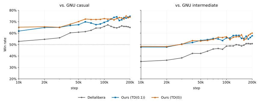
Some observations:
-
50k-100k games are enough to get most of the performance
-
TD($\lambda=0$) and TD($\lambda=0.1$) are similar
-
running for longer doesn't improve win rate much. We don't show it here, but if you run for 10x longer (2M games), then we don't meaningfully improve vs. intermediate.
Play against the agent
Since the model is so small, we can run it in the browser! Below is a local implementation. You may also open the game in its own page.
The model was trained with '1 ply' i.e. no search, but you can run with up to '3 ply' here.
References
Appendix
Encoding
Backgammon can be encoded very tersely. Here is an example board state,
+-----------------------+---+-----------------------+ +-----+
| 13 14 15 16 17 18     |   | 19 20 21 22 23 24     | | OFF |
+-----------------------+---+-----------------------+ +-----+
|  V  v  V  v  V  v     | B |  V  v  V  v  V  v     | | X X |
|  X  .  .  .  O  .     | A |  O  .  .  .  X  X     | | X X |
|  X  .  .  .  O  .     | R |  O  .  .  .  X  .     | | X   |
|  X  .  .  .  .  .     |   |  .  .  .  .  .  .     | |     |
|  .  .  .  .  .  .     |   |  .  .  .  .  .  .     | |     |
|                       |   |                       | |     |
|                       | X |                       | |     |
|  .  .  .  .  .  .     |   |  .  .  .  .  .  .     | |     |
|  .  .  .  .  .  .     |   |  .  .  .  .  .  .     | |     |
|  O  .  .  .  .  X     |   |  O  O  .  .  O  .     | |     |
|  O  .  .  .  .  X     |   |  O  O  .  .  O  .     | | O   |
|  A  a  A  a  A  a     |   |  A  a  A  a  A  a     | | O O |
+-----------------------+---+-----------------------+ +-----+
| 12 11 10  9  8  7     |   |  6  5  4  3  2  1     | | OFF |
+-----------------------+---+-----------------------+ +-----+
All we need to track is how many checkers are at each of the 24 points, how many are on the bar, and how many have been borne off.
We can do this with an array, state, of length 28,
- indices
0..23represent the points.state[i] = +nif player 0 hasncheckers at pointi,-nif player 1 hasncheckers; - indices
24, 25count how many checkers player 0 and 1 (resp.) have on the bar; - indices
26, 27count how many checkers player 0 and 1 (resp.) have borne off.
That's it!
We also need a feature vector to pass to the neural network. We start with some indicator features for each point,
for i in 0..23:
  for n in 1..3:
    for p in 0..1:
      f_point[i,n,p] = 1 if point i has at least n checkers belonging to player p
We also count how many checkers a point has above 3
for i in 0..23:
  for p in 0..1:
    n = max(state[i] * (1 if p == 0 else -1), 0)
    f_point_above_3[i,p] = max(n - 3, 0) / 2 # scaling is arbitrary
We finally count how many checkers each player has on the bar and has borne off,
for p in 0..1:
  f_bar[p] = count(player p has on the bar) / 2
  f_off[p] = count(player p has borne off) / 15
# scale these features to be <= 1 (total checkers per player is 15)
This gives 24*3*2 + 24*2+ 2*2 = 196 features in total.
Glossary
Equity- expected number of points. In Backgammon you can score 2 points for a gammon (bearing all your checkers off while the opponent has borne off no checkers), 3 points for a backgammon (a gammon where the opponent has at least one checker on your home board or on the bar), or 1 point for bearing off first. This means your equity can be between-3and+3.n-ply- a ply is a turn taken by a player in a game. In the context of game-playing algorithms, we might say that an algorithm is '3-ply', which means the algorithm searches 3 moves ahead when making its decision. Confusingly, people index their plies differently, so some write 'n-ply' to mean 'n+1-ply'